OpenFOAM: pimpleFoam w HEAT TRANSFER -1

This post is the first of two that a record of how to modify the pimpleFoam solver of OpenFOAM to include heat transfer when there is: a porous region, two phases (gas and solid = porous region), and a heat source within the solid region. In this post, a single energy (T) equation is added for the fluid phase. In the next post, the second energy (T) equation is added for the solid phase. This also requires that the two phases are linked and that porous region is defined. The assumptions of pimpleFoam (incompressible, turbulent, transient) are also adopted. This was written at the start of 2022, with OpenFOAM v9 used. This post is the second of two that a record of how to modify the pimpleFoam solver of OpenFOAM to include heat transfer when there is: a porous region, two phases (gas and solid = porous region), and a heat source within the solid region. In the first post, a single energy (T) equation was added for the fluid phase. In this post, a second energy (T) equation is added for the solid phase. This also requires that the two phases are linked and that the porous region is defined. The assumptions of pimpleFoam (incompressible, turbulent, transient) are also adopted. This was written at the start of 2022, with OpenFOAM v9 used. The porous region is a pile of sugar beets in the field – a “clamp”.

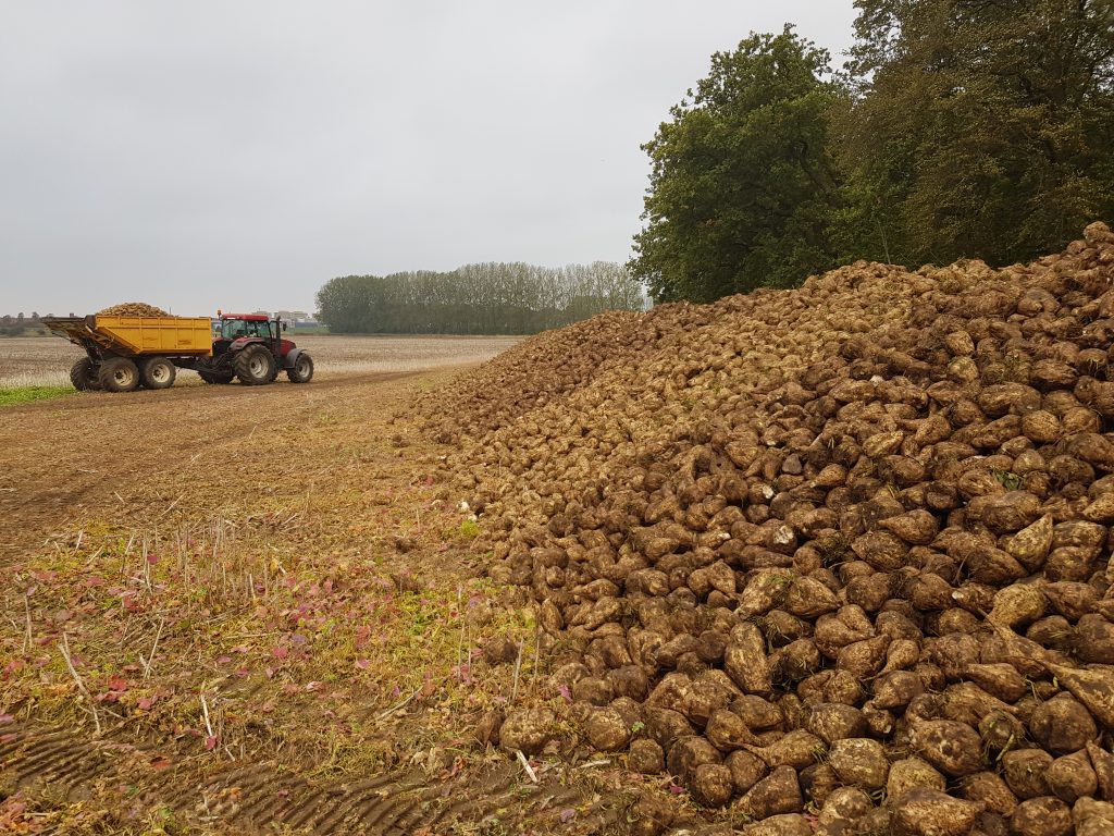
t’s a 2D simulation. From a simulation of air flow, the porous region looks something like this, with the full domain extending out 5m in all directions:

Why two posts? Two reasons: 1. it would be too long as one, and; 2. it’s good practice to build code up in stages so that bug detection is easier.

Everything in this post is sourced from elsewhere, including; the course by Håkan Nilsson (Chalmers), a blog post by Andrea De Santis on adding a single passive scalar transport equation (temperature) to pimpleFoam, an article and corrections from my co-author Morteza Mousavi, and few others at the Department of Energy Sciences, LTH, Lund. I recommend Andrea’s blog as the starting point if you are like me and have some basic knowledge of OpenFOAM and just want to get a solver that works for that set up. Håkan’s course gives you the knowledge to elevate yourself to OpenFOAM pro and start making any change to the code you like.

Contents:

governing equations
getting set up
adding parameters to application
adding governing equations
compile the solver
test it all

1. GOVERNING EQUATIONS

Just for reference:

Mass

(1) $\begin{equation*} \nabla.U = 0 \end{equation*}$

Momentum

(2) $\begin{equation*} \frac{\partial U}{\partial t} + \nabla . (U U) = -\nabla p + \nabla.\tau + S \end{equation*}$

where

(3) $\begin{equation*} \tau = \mu (\nabla U + \nabla U^T) -\frac{2}{3}\mu I(\nabla . U) \end{equation*}$

and

(4) $\begin{equation*} S = -(\mu D + \frac{1}{2} \rho U F) U \end{equation*}$

The momentum equation is just the incompressible Navier-Stokes equation. These two balance equations are already implemented within the pimpleFoam solver. The porous medium, including the Darcy and Forchheimer coefficients, is implemented from the fvOptions file.

The governing equation to be added to the solver is for temperature.

(5) $\begin{equation*} \epsilon (\rho Cp)_f \frac{\partial T_f}{\partial t} + \epsilon (\rho Cp)_fU.\nabla T_f = \epsilon \nabla.(k_{f}\nabla T_f) \end{equation*}$

There is a bit going on here, and some further description is needed.

To start with, the f subscript – for “fluid” – is added to everything in preparation for there being a second $T$ .

$\epsilon$ is the porosity. This will be 1 in the air space around the clamp, and around 0.45 in the porous zone. From a ‘common sense’ point of view, this needs to be added to reduce the rate of heat transfer as there is simply less air in this porous region and so the amount of heat that is transferred within the fluid phase must be less than in the open air. From a mathematical point of view, it looks superfluous – divide through by $\latex \epsilon$ and it disappears. It remains there for now as in the next post, an extra term is added to this equation that is not a function of porosity.

The specific heat of air $Cp_f = 1005$ J/kg.K. Density $\rho = 1.225$ kg/m³.

As the fluid phase is turbulent, $k_f$ needs to be considered as $k_{eff_f}$ – the effective thermal conductivity of the fluid phase, which is the combined molecular conductivity and the extra conductivity from the thermal mixing caused by the turbulence. This is where the algebra gets fun. The $\rho Cp$ coefficients on the time derivative and convective parts (the first two parts) of the governing equation are both, well, on both parts, clunky, and unnecessary. It also turns out that $\frac{k}{ \rho Cp}$ neatly captures the idea of thermal diffusivity, and is usually given as $\alpha$ . It also turns out that $\alpha = \frac{k}{ \rho Cp} = \frac{\nu}{Pr}$ . That is, the kinematic viscosity divided by the Prandtl number for the given fluid. And then, there is a turbulent equivalent of the thermal diffusivity which can be given as $\alpha_t = \frac{\nu_t}{Pr_t}$ . So, the effective thermal diffusivity $\alpha_{eff} = \alpha + \alpha_t = \frac{\nu}{Pr} + \frac{\nu_t}{Pr_t}$ . And don’t forget the porosity constant.

Three of these values are well described for the fluid of air: $\nu = 1.38e-5$ at 5 degrees C, $Pr = 0.73$ , and $Pr_t = 0.9$ . $\nu_t$ varies with turbulence rates and thus must by calculated across the whole domain within the solver.

This also means that the temperature equation can now be given as

(6) $\begin{equation*} \epsilon \frac{\partial T_f}{\partial t} + \epsilon U.\nabla T_f = \nabla.(\epsilon \alpha_{eff_f}\nabla T_f) \end{equation*}$

A summary of all this is included in section 3 below. For now, we turn to getting setup with the pimpleFoam solver.

2. GETTING SET UP

Following the recommendations of everyone, the solver will be developed within the user profile. I can’t remember exactly if the required directories are in the user profile by default, but you want to copy the directories that OpenFOAM has. In particular, “run”, “applications” and “src”. Check if you have these using the list (ls) command with the alias for the user directory. I think you should at least have “run”

ls $WM_PROJECT_USER_DIR

Nothing there? Only “run”? Then use the make directory (mkdir) command (or, as given, make directories) including the parent directories (-p)

mkdir -p $WM_PROJECT_USER_DIR/{applications/solvers,src}

Move into applications/solvers using the change directory (cd) command

cd $WM_PROJECT_USER_DIR/applications/solvers

Create a duplicate of the original pimpleFoam solver using the copy (cp) command. Take all the sub-directories (-r = recursive), from its current directory, and into your current directory (the “.” at the end).

cp -r $FOAM_APP/solvers/incompressible/pimpleFoam .

Rename the solver and the files within it so that there is no chance for confusion between your new solver and the original. Use the move (mv) command, stating which file to ‘move’ including its path, then stating where to move it to and under what name. In this example, the path is the current directory, so that part is not stated. I’m calling this solver clampPimpleFoam – probably a bad choice (non-descriptive, not going to be easy to name extended versions) but it’s short

mv pimpleFoam clampPimpleFoam

And then do the same renaming for everything inside your newly renamed directory. There is the easy way, which involves (installing then) using the rename command

sudo apt install rename
rename 's/pimpleFoam/clampPimpleFoam/' *

But given I don’t have sudo permission on the work computer, I can’t find an alternative workable solution, and I only have one file with pimpleFoam in the name, I did this step manually in a text editor. The alternative looks like it would be based on the find and xargs or exec commands.

There is a directory that came with move that we don’t need, so it is removed

rm -r clampPimpleFoam/SRFPimpleFoam

And then, the last bit of gardening: we need to ensure that the files that will take our new solver from a bunch of text files into an executable application – the Make files – refer to this new directory and the renamed files in it. That is, in the file /Make/files, change “pimpleFoam” to “clampPimpleFoam”, and “FOAM_APPBIN” to “FOAM_USER_APPBIN”. This is easily done in a text editor but more safely done with the find and sed commands

find . -type f -exec sed -i 's/pimpleFoam/clampPimpleFoam/g' {} +

and

find . -type f exec sed -i 's/FOAM_APPBIN/FOAM_USER_APPBIN/g' {} +

Note that because the “.” path was used and the current directory is /solvers, these commands will change the instances of ‘pimpleFoam’ and ‘FOAM_APPBIN’ in all the files in all the sub-directories. It appears to not have been a problem, but it would have been safer to changed directory into solver/clampPimpleFoam/Make before running these commands.

The options file doesn’t need to be changed (yet). For reference, this file points to a heap of OpenFOAM base files (mainly in $FOAM_SRC) that will ultimately be included in the solver application. A good description of the Make process can be found somewhere in Håkan Nilsson’s course.

3. ADDING PARAMETERS TO SOURCE CODE

The temperature governing equation (eq 6) include the following parameters:

$T_f =$ temperature of the fluid : scalar field
$\epsilon =$ porosity : scalar field
$\alpha_{eff_f} =$ thermal diffusivity with the fluid phase : scalar field

To get $\alpha_{eff_f}$ , we need:

$Pr =$ Prandtl number : dimensioned scalar
$\nu =$ kinetic viscosity : dimensioned scalar
$Pr_t =$ turbulent Prandtl number : dimensioned scalar
$\nu_t =$ turbulent kinetic viscosity : scalar field

These all need to be added to the source code as things that exist in the system. When adding such parameters to the code, some programming languages would call these parameters “dimensions”, others “variables”, and others something else (“parameters” maybe). The closest open OpenFOAM seems to come to a collective noun for them is the term “objects”. But in the documentation it is more common to call them by what type of algebraic objects they are, using linear algebra parlance. They are created through the file solver/clampPimpleFoam/createFields.H. As listed above, everything is a scalar, and either a field or is ‘dimensioned’. Note though that $\nu$ is already included in the pimpleFoam system (somehow).

DIMENSIONED SCALARS

Dimensioned scalars seem to be OpenFOAM speak for what a commoner might call “a fixed number”. All the dimensioned scalars listed here will be read into the model through the createFields.H file and also be listed and quantified in the CASE/constant/transportProperties case file. One line could be added to the createFields.H file for each dimensioned scalar. Alternatively, given there are a few of these now, and more in the near future, a separate readTransportProperties.H file can be created and referenced within the createFields.H file. This is what is done here. Again, note that $\nu$ is already included in the pimpleFoam system (somehow), but also note that its value still needs to be user defined in control/transportProperties.

Using a text editor, in createFields.H, find the line

singlePhaseTransportModel laminarTransport(U, phi);

and replace it with

#include "readTransportProperties.H"

CREATE FIELDS

Still in your text editor, create a new file and save it as solver/clampPimpleFoam/readTransportProperties.H . Add in all the extra dimensioned scalars that are to be defined in CASE/constant/transportProperties. The dimensioned scalar just removed from createFields.H also needs to be added, but, again, $\nu$ is already in there (somehow). So:

// 
singlePhaseTransportModel laminarTransport(U, phi);
// Prandtl number - fluid:fluid [-]
dimensionedScalar Pr("Pr", dimless, transportProperties);
// Turbulent Prandtl  number - fluid:fluid [-]
dimensionedScalar Prt("Prt", dimless, transportProperties);

TRANSPORT PROPERTIES

Now, these new dimensioned scalars, with their values, need to be added to the CASE/constant/transportPropeties file. The full (post-header) transportProperties file now reads:

transportModel  Newtonian;

nu [0 2 -1 0 0 0 0] 1.382e-05; // 5 degree C
Pr 0.73; // Prandtl number
Prt 0.9; // Turbulent Prandtl number

DIMENSIONED SCALARS

Back in createFields.H, we can now add in the scalar fields: $T_f$ , $\epsilon$ , and $\alpha_{eff_f}$ . The $\alpha_{t_f}$ field will also be added as part of the calculations. Just like $\nu$ , $\nu_t$ is already in the pimpleFoam system. Given the absence of Greek letters on the keyboard, $\epsilon$ is named in the OpenFOAM code as “por”, $\alpha_{eff_f}$ is renamed as “aefff”, and $\alpha_{t_f}$ is renamed as “atf”. The following is added to the file below the two existing volScalarFields (p and U).

volScalarField Tf
 (
     IOobject
     (
         "Tf",
         runTime.timeName(),
         mesh,
         IOobject::MUST_READ,
         IOobject::AUTO_WRITE
     ),
     mesh
 );

volScalarField por
 (
     IOobject
     (
         "por",
         runTime.timeName(),
         mesh,
         IOobject::MUST_READ,
         IOobject::AUTO_WRITE
     ),
     mesh
 );

volScalarField aefff
 (
     IOobject
     (
         "aefff",
         runTime.timeName(),
         mesh,
         IOobject::MUST_READ,
         IOobject::AUTO_WRITE
     ),
     mesh
 );

volScalarField atf
 (
     IOobject
     (
         "atf",
         runTime.timeName(),
         mesh,
         IOobject::MUST_READ,
         IOobject::AUTO_WRITE
     ),
     mesh
 );

A good description of what the code inside the volScalarField means is provided by Håkan Nilsson, lecture 9 (2020), slide 32. Basically, you’re creating the field, attaching it to your mesh, and getting it ready to run in the solver. IOobject stands for (I believe) Input/Output Object.

0: INITIAL AND BOUNDARY CONDITIONS

As these IOobjects have the “MUST_READ” flag attached, they also need a file in the CASE/0 directory, which the solver can read to get the initial and boundary conditions. The text of these is a bit long to put in this post. Instead, visit the case set up in the GitHub repository for this project.

SET FIELD

There is one more file that needs to be looked at before everything is added to the source and thus the solver can be updated, compiled, and run. The porosity has been set in the /0/por file at an initial value of 1 everywhere in the domain – it may as well be a dimensionedScalar. This is only the right value for the air space. In the porous region, it has been given as 0.45. This is changed with the setFields command. The setFieldsDict file used by this command takes a similar form as a topoSetDict. At least, the second command uses the same alternatives to define a region as does the topoSetDict. This file doesn’t need to be changed, but it’s an important part of the process. Note that this command only works because a cell set for the porous region has already been defined using topoSet and a topoSetDict.

4. ADDING GOVERNING EQUATIONS

It seems that good practice is to separate each of the governing equations out into its own .H file and then get the solver .C file to call/ reference/ include these .H files. This .H file now need to created for Tf, using our favourite text editor. For equation 6 – Temperature in the fluid phase – the .H file will be named TfEqn.H. In this file, the aefff and atf are also computed. Note that atf references “nut” and “Prt”. Prt was defined earlier, but nut is the field for $\nu_t$ , which was previously noted as included in the pimpleFoam solver already. The only issue here is that this means it is important to ensure the CASE/0/nut file exists.

// Solve the temperature equation for the fluid phase
{
     atf = turbulence->nut()/Prt;
     atf.correctBoundaryConditions();
     aefff = turbulence->nu()/Pr + atf;
     fvScalarMatrix TfEqn
     (
         por*fvm::ddt(Tf)
         + por*fvm::div(phi,Tf)
         - fvm::laplacian(aefff*por, Tf)
     );
    TfEqn.relax();
    TfEqn.solve();
}

To have the rest of solver read this new file, it needs to be added to the clampPimpleFoam.C file. Quoting directly from Andrea De Santis, with updates for the names of the files used in this example: “Since the passive scalar has no impact on the resolved flow-field we will solve for its transport equation outside of the PIMPLE loop. In order to do this open clampPimpleFoam.C, add the following line:

#include "TfEqn.H"

after the closed curly bracket which ends the PIMPLE loop and immediately above the runTime.write() line and save the changes.”

5. COMPILE THE SOLVER

With everything ready to run through the compilation process, we just need to run the compliation wmake command. This process is already set to go because the development was done inside the old pimpleFoam system and those two small changes to the Make files were made back at the end of step 2. In the terminal:

wmake

If you want to get rid of the newly compiled solver for some reason, like you realised something needs to be changed because you got an error half way through the make process, run wclear.

6. TEST IT ALL

Starting from the start, but using the files available for the case on GitHub:

Do all of the above.
Save the CASE in your USER/run directory, and move into the CASE directory
in terminal, run blockMesh to construct the mesh. NB: the mesh is workable, but pretty poor in some areas
in terminal, run topoSet to define the clamp region as a cellZone
in terminal, run setFields to set the porosity of the clamp region
in terminal, run clampPimpleFoam to run the simulation.
- this will only run a simulation of 30 seconds, and the time step is set as 0.001, so it will still take a while. Change the details in controlDict if you want it to run in another way (I couldn’t get a variable time step to work – it raced to 1 second, but diverged on k and/or epsilon).
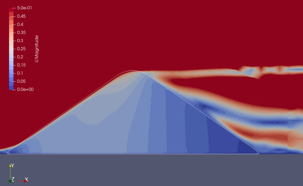
- the temperature field has an initial vale of 278K, and the inlet (left) is set to a constant 300K. The air is set at a constant (5, 0, 0), that is, 5m/s left to right.

30 seconds of simulation ends up something like this:

30 seconds of simulation. The initial blue area is 5 C, and the red wave that come in is 27 C.

REFERENCES

M. L. Hoang, P. Verboven, M. Baelmans and B. M. Nicolai (2004) Sensitivity of temperature and weight loss in the bulk of chicory roots with respect to process and product parameters, Journal of Food Engineering Vol. 62 Issue 3 Pages 233-243

S. M. Mousavi, H. Fatehi and X.-S. Bai (2021) Multi-region modeling of conversion of a thick biomass particle and the surrounding gas phase reactions, Combustion and Flame 2021 Vol. In Press

A. Potia (2017) Modeling Beet Pile, MSc Thesis, Delft University of Technology MSc. Chemical Engineering

M. S. M. Shaaban, R. Beaudry, B. Marks and K. Yousef (2014) Modeling Heat Profile of Sugar Beet Pile During Storage Campaign, American Society of Agricultural and Biological Engineers Annual International Meeting Montreal, Quebec, Canada 13-16 July.

L. G. Tabil, M. V. Eliason and H. Qi (2003), Thermal Properties of Sugarbeet Roots, Journal of Sugar Beet Research, Vol. 40 Pages 209-228

NOTE TO READER

If anyone is finding these instructions a little dumbed down, it’s because I’ve written (and rewritten and rewritten) them primarily for the dummy who will be referring to them most – myself. I’m not a professional CFD practitioner. I’m not even an engineer…

OpenFOAM: pimpleFoam w HEAT TRANSFER -1