METHODS
The methods applied in this research project include both replicated field trials including laboratory testing (Paper I and II, and SSs), replicated modified environment experiment (Paper III), and mechanistic numerical modelling employing Computational Fluid Dynamics (CFD, Paper IV). The CFD modelling includes unique data sourced from a field survey, mathematical modelling, and laboratory experimentation.
Experimental design
Field trials including laboratory testing (Paper I and II, and SSs)
Investigating the role of the availability of nitrogen and water during the growing season on the mechanical properties of sugar beet roots (Paper I), the assessment of a methodology for use of a handheld penetrometer to assess the mechanical properties of sugar beet roots (Paper II), and the initial fall-test (SS1 – falling-beet) all relied on the same field trials. Field trials of sugar beet were established during 2018 and 2019 in Sweden, the Netherlands, and Belgium. The same three varieties were grown in all trials. Three treatments were applied in six replicates, for a total of 54 plots per site. In the Netherlands and Belgium, the treatment consisted of a ladder of applied nitrogen, at rates of; no additional nitrogen, the recommended application rate, and a high application rate equivalent to the recommended rate plus 80 kg/ha. In Sweden, available growing season water was the focus. The treatment levels were defined as; no supplementary water, optimal water availability for plant growth, and wet during the last month prior to harvest. These treatments were chosen as they represent two of the key agronomic inputs to the growth of the sugar beet crop. The choice of available water in Sweden was born from many observations in industry where irrigated crops seemed to suffer from relatively high losses of quality after very long post-harvest storage periods. Each plot was split into a quality assessment section, and a mechanical properties and post-harvest storage loss assessment section.
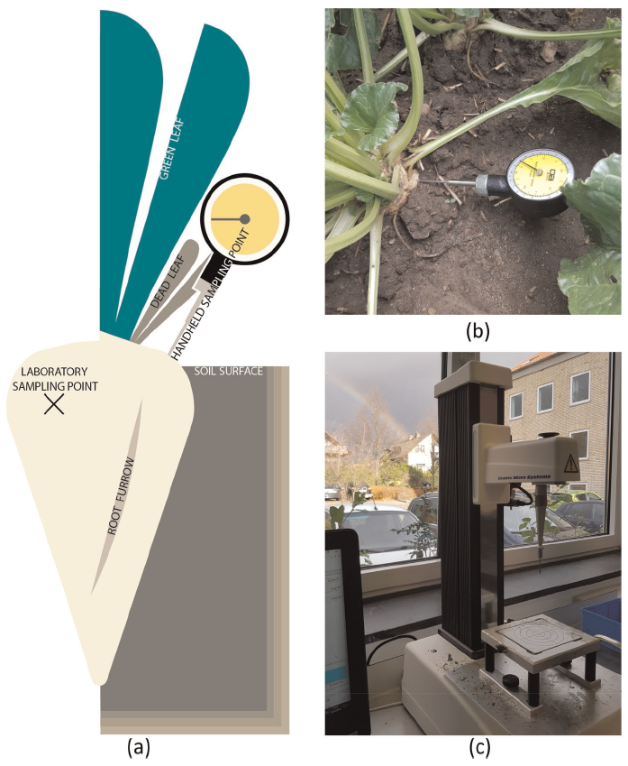
The validation of a method for the application of a handheld penetrometer in-field for sugar beet roots (Paper II) focused on a specific method that had been developed through exploratory work and through a study of the literature. The aim of this method was to be repeatable across as many growing conditions, varieties, and time periods pre- and post-harvest as possible. The method tested stated that the penetrometer should be applied at the same speed, always perpendicular to the root surface, and high on the root but below stem growth (Figure 4). It was only assessed during 2019. The falling-beet test (SS1) also occurred only in 2019 and drew only a subsample of the available plots. Within SS1, an additional sample of large and small roots was taken from a commercial field to test the role of root size in the falling-beet test.
The assessment of the second fall-test method (SS2 – falling-ball) also included a re-assessment of late season water availability. A single trial site with four replicates was established during 2021. Three agronomic treatments focused on water availability were applied in the final two months prior to harvest: natural rainfall (untreated), heavy irrigation 25 and one day prior to harvest (irrigated), and the exclusion of additional water (grown under a roof – roof). A fourth, post-harvest focused, treatment of natural rainfall plus stored under high airflow conditions was included (ventilated). This treatment was similar to the highest airflow treatment of Paper III, with a seven day duration at the highest airflow rate.
Modified environment experiment (Paper III)
Investigating the impact of airflow, temperature, and humidity on the movement of water and on quality parameters in sugar beet roots stored post-harvest in bulk (Paper III) was conducted in a modified atmosphere. The desire to use commercially harvested roots while minimising variation in the harvested material required a large experimental system. A custom built system with one primary and three secondary distributors was constructed (Figure 5. Originally Paper III, Figure 2. See also Paper III Figure 1).
Each secondary distributor had 16 ventilation boxes attached, which, with the zero airflow control ventilation boxes, gave a total of 64 ventilation boxes in the system. It was not possible to house this large system in the available controlled atmosphere chambers, so a modified atmosphere chamber was constructed. Four factors were modified and monitored: temperature, humidity, airflow rate, and ventilation duration. Airflow rate was fixed at 11.2, 46.5 and 81.5 m3/h per ventilation box. These are the levels that would be expected at 1.5, 1.0 and 0.5 meters from a ventilation pipe in a clamp when using the ventilation system developed in the NBR managed European Innovation Program project “Ventilation of sugar beet and potato stored in clamps” (Jordbruksverket project 2017-2390, (Ekelöf & English, 2022)). These are relative airflow rates of 1, 4 and 7. A zero airflow rate control was included. These airflow rates were applied in every run.
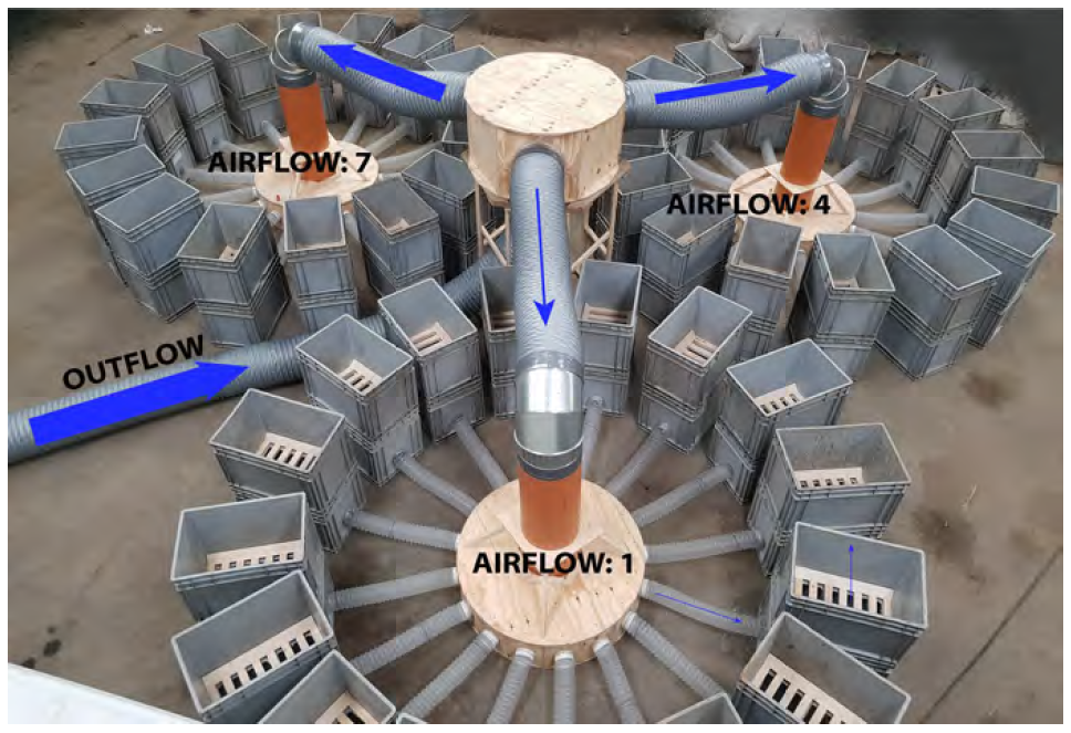
Each airflow rate was sampled at one, four and seven days, in four replicates. This meant that various combinations of total airflow volume were repeated in the experiment, e.g. 1 day at airflow rate 7 gives the same total airflow volume as 7 days at airflow rate 1. Ventilation boxes were back-filled to maintain the airflow conditions. Roots included in the back-fill after one day were also used to assess changes to density. For each airflow level, four additional ventilation boxes were filled by two reference samples of each of washed roots and soil sampled at harvest (Figure 3, Paper III). The experiment was planned to run for six one week runs, but the decision was taken to abandon the third run (week three from the first harvest). This was based on signs of advanced quality loss in the bulk of roots that the samples were picked from. The majority of roots had visible mould growth. For each run, target temperature and humidity conditions were set, with actual values recorded at 15 minute intervals. The targets were set to give a range of conditions that are commonly found during post-harvest storage in Sweden. The final temperature and humidity conditions were quite stable, but somewhat limited in the coverage they gave.
Computational Fluid Dynamics modelling (Paper IV)
The spatial-temporal numerical model of airflow and temperature (Paper IV) was developed using a modelling structure built on standard Computational Fluid Dynamics (CFD) methods but to the specific requirements of the system being modelled. This model was always intended to be the first step in a long process of model develop, and as such was developed to build a foundation, not as a model of high refinement. The model uses the finite volume method and a porous medium approach. Governing equations for a transient, turbulent, and incompressible system were defined, given below in Equations 1 to 6.
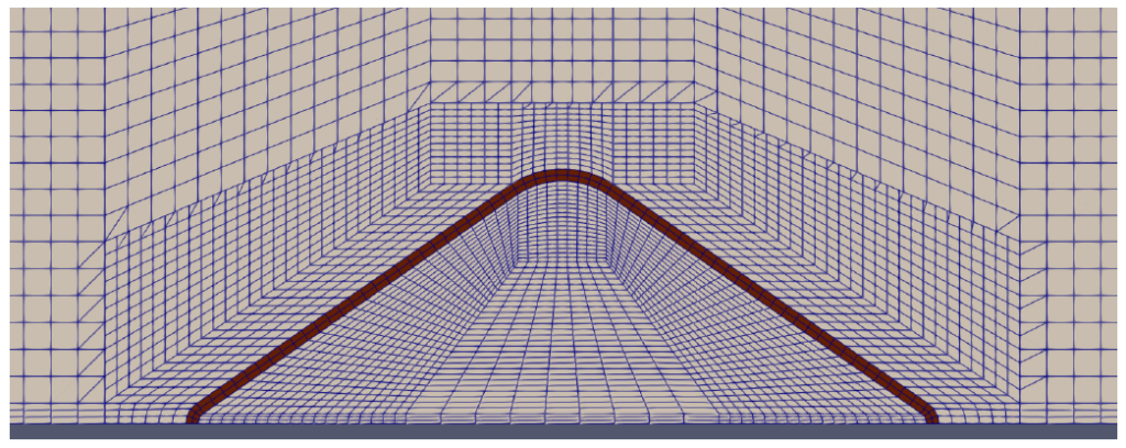
In the finite volume approach, the model domain is divided up into small cells (Figure 6). The governing equations are also known as balance equations, as they state that for any given cell of the model, the mass of, momentum of, or energy in the fluid must remain in balance. Because of the assumption of an incompressible flow and the finite volume method, the equation for mass (Equation 1) says that the net rate of change in flow of velocity through the walls a cell in the x, y and z axes must equate to zero. The Nabla operator, ∇, symbolises the words “net rate of change … along the x, y and z axes”. It is here the divergence: the vector field equivalent of a derivative. If you were to think of one of the ventilation boxes shown in Figure 5, Equation 1 says that the total amount (mass or volume) of air flowing in through the pipe in the side wall (along the x-axis) must be equal to the total amount of air coming out the open top (along the y-axis). The equation for momentum (Equation 2) – which is the equation for airflow – states that the change in momentum over time will be equal to the net changes from convection, pressure, viscous forces, and any forces coming from within the volume. The equation for the temperature of the air (Equation 6) states that any changes in the temperature of the air over time will result from the convection of air, conduction within the air, and transfers between the sugar beet roots and the air. Finally, the equation for the temperature of the sugar beet roots (Equation 5) states that any changes in the temperature of the sugar beet roots over time will result from conduction within the roots, transfer between the sugar beet roots and the air, and from the heat of respiration. The transfer of temperature between the sugar beet root mass and the air depends on the surface area within the cell, the resistance of the surface to the transfer of temperature, and the difference in temperature between the air and the roots. The heat of respiration is defined to depend on the temperature of the roots. More formally, the governing equations are given as:
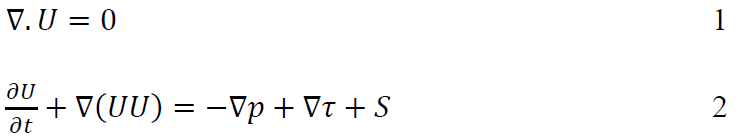
where U is the vector for velocity, t is time, p is pressure, and τ is the convective stress tensor. The standard k-epsilon model of turbulence is applied. The source term is used in the porous medium approach to capture the loss of velocity that occurs as air moves through the porous bulk. The source term S is here defined as the Darcy-Forchheimer equation for a homogeneous porous media:

where D and F are scalars. The Darcy (D) component of the source term captures viscous loss and is linearly proportional to the velocity, while the Forchheimer (F) component captures the inertial loss and is proportional to the velocity squared.
It is assumed that heat transfer from radiation is negligible within the entire system. Heat transfer is assumed isotropic. Within the solid phase (the sugar beet roots), it is assumed that there is thermal equilibrium and no convection. The energy equations for the fluid (f) and solid (s) phases are given for temperature (T) as:
As the fluid phase is turbulent, 𝜀(𝜌 𝐶𝑝)𝑓 can be given as 𝛼𝑒ff (see Paper IV, Section 2.3.5). This allows Equation 4 to be stated as:

Where ε is porosity, ρ is density, Cp is specific heat, K is thermal conductivity, Asf the specific surface area, hsf is the convective heat transfer coefficient, and Qr is the heat of respiration. The parameters are summarised in Paper IV, Table 1 and expanded upon throughout Paper IV. Model parameters were drawn from literature and new experiments. New data on the permeability (D and F) of the non-woven polypropylene cover used on sugar beet clamps employed an ISO standard laboratory testing procedure of the relationship between pressure and velocity of air through the material (Paper IV, Supplementary material, S1.2). New data on the dimensions of harvested sugar beet roots was sort to define Asf. This employed a survey approach, coupled with a simple mathematical model of the root (Paper IV, Supplementary material, S2). A modified version of Qr was developed to better suit the physiology of sugar beet respiration (Paper IV, Supplementary material, S3).
The model was developed as a more efficient two-dimensional model as it was assumed that the loss of information in comparison to a 3D model would not result in a loss of understanding of the general phenomena under investigation. For discretisation to a numerical model, a second order linear-upwind scheme was applied to the velocity field, and first order linear or upwind schemes applied elsewhere. The model solution was validated against experimental data from previous research conducted by NBR during the 2011-12 storage period (Olsson, 2013a). A sensitivity analysis was conducted to explore how the model solution depended on key parameters around which there was uncertainty.
Open source software was deliberately used to ensure both that the model could be tailored as required, and that it is accessible to all. The model development process was incremental, with the first model included in the final publication being model clamp_43. Many of the first 42 models were refined and rerun without the allocation of a new model number. It was found that the model would gain accuracy and efficiency by having the momentum and the energy equations (air velocity and temperatures) solved separately. The momentum equation was solved first for a 90 second period to obtain a stable solution. This solution was then passed to the energy equation solver as fixed fields. The experimental data the model was to be verified against and the available weather data were in 15 minute intervals and thus the model also progressed in this increment. A somewhat unique feature of this model within the domain of modelling post-harvest storage systems was that the system is outdoors. The major feature this introduces is constant change in the direction of airflow. This was accommodated by creating a symmetrical model domain (Paper IV, Figure 3), taking the normal component of the air velocity as the inlet velocity, and by permitting the inlet and outlet of the model to swap for any progression of the model. Radiation is another phenomena that was considered as important in this environment, but it was ultimately not included in this version of the model.
Assessment
Quantifying quality
As described in Section 1.2, storability is assessed against quality. Sugar beet root quality was assessed in Papers I and III. For Paper I, assessment was made in the laboratories of the German national sugar beet research centre in Göttingen, Institute of Sugar Beet Research (IfZ-Göttingen). For Paper III, assessment was made at the Nordic Sugar factory at Örtofta, Sweden. Assessment was completed to the same International Commission for Uniform Methods of Sugar Analysis (ICUMSA) standards. Sucrose concentration was determined polarimeterically (ICUMSA Method GS6-3, (ICUMSA, 1994)), amino nitrogen content via the “blue number” (ICUMSA Method GS6-5), sodium and potassium content by flame photometry (ICUMSA Method GS6-7), and dry matter content via drying to a stable weight. In Paper I, total invert sugar content was assessed via glucose content, and alcohol insoluble residues (AIR) via alcohol extraction and filtration. Alcohol insoluble residues is a measure of the cell wall content of the root (van Soest et al., 1991). In Paper I, the marc content was also measured, via water and acetone extraction (Reinefeld & Schneider, 1983) and is described as an estimate of the pulp content of a sample. In Paper III, additional metrics of quality were included. The final dirt-tare was assessed at Örtofta as the percentage of weight washed away during cleaning. The effect of ventilation on the weight cleaned from the roots post-ventilation was assessed as the loss of weight when the roots were put through a simulated cleaning (Paper III, Figure 4). The volume of the individual roots used in the calculation of changes to density was assessed by weighing the mass of water displaced during immersion.
Quantifying mechanical properties
The laboratory measurement of mechanical properties of sugar beet roots (Papers I and II) followed the method developed in Kleuker and Hoffmann (2019). This includes the three metrics of puncture resistance, tissue firmness, and compression strength. Puncture resistance and tissue firmness are both measured with a 2 mm diameter cylindrical probe (Figure 4c), inserted at a speed of 1 mm/s into an entire root at its widest diameter, to a depth of 5 mm. Puncture resistance is the maximum pressure recorded as the probe pierces the periderm of the root, and tissue firmness the average pressure from approximately 0.5 mm after puncture through to 5 mm (see example pressure-distance output from penetrometer in Figure 9). Compression strength is measured with a flat plate also moving at a speed of 1 mm/s, on an 18 mm diameter core taken from a 20 mm slice from the widest diameter of the root. In SS2, a laboratory penetrometer was used but only with a probe. The apparent modulus of elasticity in SS2 was assessed as the average slope of the curve to puncture. It is termed “apparent” as the elastic behaviour of the root is not actually allowed to express.
The assessment of the accuracy of the method adopted for the handheld penetrometer (Paper II) was made in relation to the laboratory equipment. The first test of the method was whether it gave the same general patterns. The statistical analysis focused on the correlation between the results from the two penetrometers. The efficiency of the handheld method was also an important consideration. This was assessed on the number of samples needed to find stable results, the variation in results between operators, and on the time it took to take the required number of samples. The application of the handheld penetrometer in Paper III followed the method developed in Paper II.
Measurement of dynamic impacts
In SS1, sugar beet roots were dropped from one meter onto a 10 mm thick smooth plastic plate sitting on a concrete floor. It was felt that dropping the root would give flexibility in adjusting the drop height, and would capture the actual force at impact and how it is distributed. The force of impact is measured as impulse:
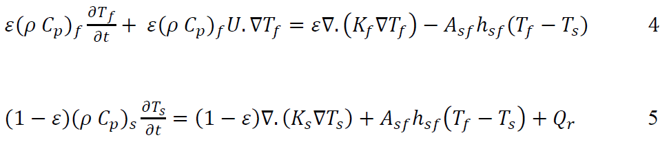
where: t1 = 0, and is the point when the root makes contact with the plastic plate; t2 is the time at which the downward movement of the root stops; m is the root mass; and Δ𝑣𝑣 is the change in velocity during contact. Identifying t2 was achieved with a high speed camera (960 frames per second, Samsung S10). Velocity at t1 was calculated based on drop height and acceleration from gravity. Velocity at t2 is zero, and therefore Δ𝑣𝑣 = 𝑣𝑣𝑡𝑡1 . Mass was measured prior to the drop test. To translate the average force of impact to average pressure at impact, the area of impact was measured as a carbon paper transfer captured at impact (Figure 7) with image analysis conducted in Adobe Photoshop. The practicality of the method was assessed subjectively.
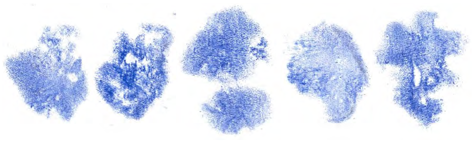
In SS2, the fall was inverted, with the root fixed in a bulk of sand and a 70 mm diameter, 1.4 kg steel ball dropped on the root from a height of 0.93 m (Figure 8). The impact site was assessed for level of visible surface damage on a scale of 0-5, with 0 equal to 0 % visible damage and 5 equal to 100 % of the impact site showing damaged cells. The number and total length of cracks was measured from the centre of the impact site. Force and pressure measurements were not taken.
Modified environment conditions
The temperature and humidity of the modified atmosphere system (Paper III) was controlled with a commercial greenhouse climate control unit. Measurement of temperature and humidity was with one Hobo Pro v2 logger per airflow rate, placed in one of the boxes attached to the secondary distributors. Airflow rates were set and regularly verified using grid sampling in the inflow pipe to the secondary distributors (orange pipes in Figure 5). A Testo 405i hot wire anemometer was used.
Mass transfer, water vapour deficit, convective mass transfer coefficients, diffusivity
In the modified atmosphere experiment (Paper III), the rate of mass transfer was reported as mass flux, 𝑚𝑚̇𝑤𝑤 [mol/m2/s]. Mass flux was taken as

where kc is the convective mass transfer coefficient and Δ𝑐 is the water vapour deficit. Mass flux was calculated as weight loss per unit surface area and time, with weight loss taken from the experiment and assumed to be just water. The surface area calculation assumed a spherical object. The diameter of this sphere was calculated via volume, which was taken as (weight of total sample) ÷ (roots per sample) ÷ (density as described in Section 3.2.1). The level of contact between the roots in the sample was not considered. Water vapour deficit was calculated using Tetens equation (Monteith & Unsworth, 2008), with the water activity of the roots taken as 98.5 % (Chirife & Fontan, 1982). The convective mass transfer coefficients calculated from the experiment were compared to estimates from dimensional analysis, using the Sherwood-Reynolds-Schmidt correlation (Carta, 2021b):

where: L is the characteristic length [m] calculated as diameter via weight, density and the assumption of a sphere; Dab is water diffusivity [m2/s]; Re the dimensionless Reynolds number; and Sc the dimensionless Schmidt number. Estimates of Dab were taken from the airflow rate 0 samples. Re is dependent on airspeed.
CFD model functionality and accuracy
Assessment of the functionality of the CFD model was based on its ability to operate without error, its speed, and inspection of the time series to assess if it behaved as expected. All parameters in the CFD model were recorded at 15 minute intervals at points in the clamp region of the model of equivalent location to the temperature loggers used in the original 2011/12 experiment. Assessment of the accuracy of the CFD model was based on the mean absolute error (MAE) of the recorded temperature time series in comparison to the experimental series. Further checks on the system of solvers were run. Mesh independence was tested on a mesh of approximately half (2688 cells) and approximately double (10752 cells) the number of cells in the mesh used in the analysis (6123 cells). Testing of the stability of the airflow field at points in the open air region was conducted to understand if there was the potential to improve the efficiency of the system of solvers and the 90 second time period applied in the solving of the momentum equation (Paper IV, Supplementary material, Figure S4.1).
Economic analysis
A single economic analysis was conducted in this research project. The impact of ventilation on the gross income per harvested tonne was assessed in Paper III using the commercial payment schedule from Sweden’s single processor for 2021.