CONVECTIVE HEAT TRANSFER IN SUGAR BEET STORES

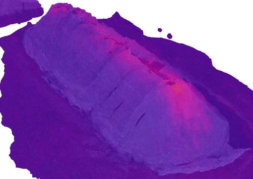
Cover image: a sugar beet clamp captured with a drone mounted thermal camera.

Skip to Coding convective heat transfer coefficient as a scalar field.

BACKGROUND

Convective heat transfer is the process by which heat is transfer from one region to another through the movement of a fluid. It results when there is a temperature difference between the two regions, and a fluid that is able to move between the regions. In a pile of sugar beet roots, convective heat transfer is the processes that occurs at the surface of the sugar beet out into the air surrounding that beet. If the sugar beet cool because they are surrounded by cooler air, it’s convective heat transfer.

In the case with the solid (sugar beet root) surrounded by a fluid (the air), the rate of convective heat transfer is determined by:

the magnitude of the temperature difference,
the total surface area between the two regions over which heat energy can flow, and
the properties of the surface that can facilitate heat transfer.

These can be given as:

temperature divergence: (T_s – T_f), or $\Delta T$ , or div.T [K]
specific surface area (A) = surface area per unit volume: [m²/m³ or 1/m]
heat transfer coefficient (h): W/(m².K)

Combining these, and the units become W/m³. Multiply that by specific heat (energy needed to raise the material by one degree), you get the change in temperature per unit volume per unit time. Temperature divergence will be time and space dependent – constantly varying within a CFD model. Specific surface area and the heat transfer coefficient will be taken as constant.

The temperature divergence will be defined in the model. The specific surface area is described in another post. The calculation of the heat transfer coefficient for sugar beet is here described.

CALCULATING CONVECTIVE HEAT TRANSFER COEFFICIENT FOR SUGAR BEET

For this attempt, in lieu of any good experimental data, the Ranz-Marshall correlation is applied. The Ranz-Marshall correlation applies a fixed equation for the Nusselt number (Nu), as a function of the Reynolds number (Re_D) and Prandtl number (Pr).

(1) $\begin{equation*} Nu = 2 + 0.6Re_D^{1/2}.Pr^{1/3} \end{equation*}$

This is equated to the full definition of the Nusselt number (convective heat transfer / conductive heat transfer):

(2) $\begin{equation*} Nu = \frac{h}{k_f/D_{eq}} = \frac{hD_{eq}}{k_f} \end{equation*}$

Where, k_f = thermal conductivity of the fluid and D_eq = equivalent diameter. So,

(3) $\begin{equation*} \frac{hD_{eq}}{k_f} = 2 + 0.6Re_D^{1/2}.Pr^{1/3} \end{equation*}$

and

(4) $\begin{equation*} h = \frac{k_f}{D_{eq}} (2 + 0.6Re_D^{1/2}.Pr^{1/3}}) \end{equation*}$

ONE AT A TIME…

k_f: THERMAL CONDUCTIVITY

Thermal conductivity of the fluid. For air at 5 C, k = 0.02474 W/(m².K)

D_eq: EQUIVALENT DIAMETER

$D_{eq} = (6V/\pi)^{1/3}$ . V = 1372cm³, D_eq = 13.786cm = 0.13786m

Pr: PRANDTL NUMBER.

In air, this is given as the constant 0.72. The turbulent Prandtl number of air is 0.90, but we’ll assume a laminar flow at the beet surface.

Re_D: REYNOLD NUMBER.

$Re_D = \frac{UD}{\nu}$ , where U is the superficial velocity, D is the diameter of the particle (= D_eq), and $\nu$ is the kinematic viscosity of the fluid. If an average U is taken as 0.1m/s, D= 0.13786m, and $\nu$ = 1.38 e-05, Re_D = 463. This should probably be incorporated into the model as a scalar field (see below).

GIVES…

h=3.407 . This is thankfully a lower value than used previously.

RESULT

Temperature of the air. 15 seconds. It takes about 8 seconds for the air in the clamp to reach the same temperature as the beets. T_f0 = 288, T_s0 = 274, T_{f_inlet} = 300

Temperature of the beets. Over 15 seconds, the change is minute. T_f0 = 288, T_s0 = 274, T_{f_inlet} = 300

h AS A SCALAR FIELD

As noted above, Re_D is a function of the superficial velocity. This superficial velocity will vary a lot across the clamp. It will pretty much always be low, but look at these numbers:

U	Re_D	h
0.01	46,3	1.19
0.10	463	5.24
0.20	926	7.10
0.30	1389	8.52
0.40	1852	9.72
0.50	2315	10.78
1.00	4630	14.92

Again, not large numbers, but there are two points to note.

Re_D is pushing towards turbulent. We’re going to assume this away for now as velocities of 1,00 will be rate inside of the porous clamp region. If we did want to account for this, I believe a different correlation can be used; instead of 6, 1/2 and 1/3 as the coefficients in the Ranz-Marshall equivalence for Nu, different values can be used.

The second point is that at the given U values, the h values (increasing at a decreasing rate) are a whole magnitude of order larger at 0.50 compared to 0.01. From the previous simulations with 5m/s inlet air speed, velocity magnitudes of 0.01 and 0.30 were found in the one clamp.

CODING h AS A SCALAR FIELD

OpenFOAM version: 9

Case: clamp_08

Solver: clampPimpleFoam-2 –> clampPimpleFoam-3

We’re again going back and modifying the solver. This has been done twice before: once with the addition of T_f and once with the addition of T_s. Note that all these versions are just referred to in controlDict and in the OpenFOAM terminal as ‘clampPimpleFoam’.

Of all the variables noted above, D_eq, Re_D and k_f don’t already exist in the solver. h is defined within the solver, but as a fixed scalar. In the solver it has the name h_sf (convective heat transfer coefficient, from the solid phase to the fluid phase). It needs to now be included as a scalar field instead.

DEFINING SCALARS IN THE SOLVER

Starting with these new scalar fields. In createFields.H, add in h_sf and Re_D to the list of other manually added scalar fields:

volScalarField hsf
 (
     IOobject
     (
         "hsf",
         runTime.timeName(),
         mesh,
         IOobject::MUST_READ,
         IOobject::AUTO_WRITE
     ),
     mesh
 );
volScalarField Red
 (
     IOobject
     (
         "Red",
         runTime.timeName(),
         mesh,
         IOobject::MUST_READ,
         IOobject::AUTO_WRITE
     ),
     mesh
 );

h_sf needs to now be removed from the readTransportProperties.H file.

With the readTransportProperties.H file open, add in k_f and D_eq:

// Thermal conductivity - fluid:fluid [W/(m.K)]
dimensionedScalar Kf("Kf", dimensionSet(1, 1, -3, -1, 0, 0, 0), laminarTransport);
// Characteristic length = Equivalent diameter of a sphere [m]
dimensionedScalar Deq("Deq", dimensionSet(0, 1, 0, 0, 0, 0, 0), laminarTransport);

CALCULATING SCALARS IN THE SOLVER

h_sf and Re_D are fields as they change with time and space. The need to be computed for each mesh cell at each time step. A new hEqn.H file is created, with the following content:

{
    Red = mag(U) * Deq / turbulence->nu();
    hsf = Kf / Deq * (2 + pow(Red, 0.5) * pow(Pr, 0.3333));
}

A line to call this new file is added in clampPimpleFoam.C (the second and third lines here already exist).

        #include "hEqn.H"
        #include "TfEqn.H"
        #include "TsEqn.H"

NB: in a latter step in the development of this model, the calculation for Qr for TsEqn.H is updated to give a different functional form. This update is incorporated in this version of the solver on GitHub.

DEFINING THE SCALARS IN THE CASE

In the case file constant/transportProperties, h_sf must also be removed and k_f and D_eq must also be added.

Kf      [1 1 -3 -1 0 0 0] 0.02474; // thermal conductivity - fluid
Deq     [0 1 0 0 0 0 0] 0.13786; //characteristic length

As h_sf and Re_D are now in the solver as input-out objects (IOobject) with the “must read” tags, they need to be defined in CASE/0. These files are in the case repository.

RESULTS

Using the updated solver and case clamp_08:

Temperature of the solid phase (sugar beets). 15 seconds. There seems to be a little more heat exchange at the edges of the clamp, with the higher velocities, when compared to the video of Ts above.

Heat Transfer Coefficient (h_sf). 15 seconds of simulation. Inlet velocity (from left) = 5m/s. Definitely variation across the clamp.

UP NEXT

Getting very close now… Once the correct data for the cover permeability is sort, it’s just a matter of getting the time series for the inlet temperature and velocity in place and we can run a full test simulation on both the uncovered and covered clamps. Oh, and implement a variable time step (but that, I believe, is straightforward). Really, a full test simulation of the uncovered clamp is but a few hours away.

CONVECTIVE HEAT TRANSFER IN SUGAR BEET STORES