OpenFOAM: pimpleFoam w HEAT TRANSFER -2

Solver: clampPimpleFoam-1 -> clampPimpleFoam-2

This post is the second of two that are a record of how to modify the pimpleFoam solver of OpenFOAM to include heat transfer when there is: a porous region, two phases in this porous region (gas and solid), and a heat source within the solid phase. In the first post, a single energy (T) equation was added for the fluid phase. In this post, a second energy (T) equation is added for the solid phase. This also requires that the two phases are linked and that the porous region is defined. The assumptions of pimpleFoam (incompressible, turbulent, transient) are also adopted. This was written at the start of 2022, with OpenFOAM v9 used. The porous region is a pile of sugar beets in the field – a “clamp”.

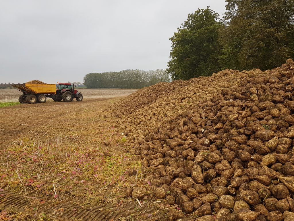
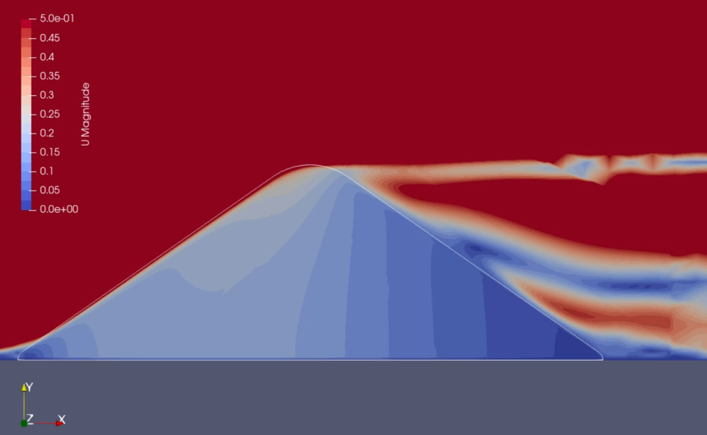
It’s a 2D simulation. From a simulation of air flow, the porous region looks something like this, with the full domain extending out 5m in all directions:

Please note that this post probably wont make a lot of sense without first visiting the aforementioned other post. There is also the warning about who the author is at the bottom of this post.

Contents:

governing equations
getting set up
adding parameters to application
adding governing equations
compile the solver
a test run

1. GOVERNING EQUATIONS

Now that a multi-phase approach is being introduced, a second energy equation needs to be added. The two phases are the air (fluid – f) phase and the sugar beet (solid – s) phase. The porous region is made up of both these phases. There is no transfer of mass between the phases – one day we’ll add in the movement of water, but not in this version. There is heat transfer between the phases, but the assumption of thermal equilibrium applies within the solid phase – something else that might be relaxed, one day. We therefore have two temperature equations:

(1) $\begin{equation*} \epsilon \frac{\partial T_f}{\partial t} + \epsilon U.\nabla T_f = \nabla.(\epsilon \alpha_{eff_f}\nabla T_f) + A_{sf}h_{sf}(T_s-T_f) / (\rho_f Cp_f) \end{equation*}$

and

(2) $\begin{equation*} (1-\epsilon)(\rho Cp)_s \frac{\partial T_s}{\partial t} = (1-\epsilon) \nabla.(k_{s}\nabla T_s) + A_{sf}h_{sf}(T_f-T_s) + Q_{resp} \end{equation*}$

There is even more going on here now, so further description is again needed.

The two equations look a little different in their set up, which is mainly because equation one – the fluid phase – was rearranged in the first post. A similar rearrangement is not necessary (possible?) for the solid phase. Equation 1 itself looks a little different from how it did in the previous post (equation 6) – there is that new term at the end, describing the heat transfer between the phases.

$\epsilon$ is the porosity. This will be 1 in the air space around the clamp, and around 0.45 in the porous zone.

BETWEEN PHASES

f and s are the solid and fluid phases respectively, with these subscripts relating to parameters of a single phase and the sf subscript relating to parameters of the transfers between the phases. It can thus be seen that the rate of transfer of heat between the phases is given as $A_{sf}h_{sf}(T_f-T_s)$ and is a function of the specific surface area ( $A_{sf}$ [m²/m³]), the difference in temperature between the two phases ( $T_f - T_s$ ), and a convection heat transfer coefficient ( $h_{sf}$ [W/m².C]). If this model wasn’t a porous medium model but a fully resolved CFD model where the two phases where physically separated as different regions in the mesh, the $A_{sf}h_{sf}(T_f-T_s)$ term would be the boundary condition. Similarly, $T_f$ would be the freestream temperature, but here will be the volume averaged value.

The value of $h_{sf}$ , well, this is the million dollar question. Mousavi (2021) has one solution that could be implemented. Potia (2017) used the value of 24.9684 W/m²K, but this was for a covered clamp in a model with no convection through the pile. There is also an estimate in Potia of 3024.6 using parameters on air flow from the air, and shape form values from beets. It may be possible to get a value for this from a past NBR project in which temperature inside of some beets was monitored. For now, we’ll just take the value from Potia (2017).

$A_{sf}$ has been modelled as part of this project. A summary is found in another blog post. For now, this figure will be taken as the constant value of 30.04 m²/m³. This feels ok: a value of 47.0 m²/m³ was used for chicory roots by Hoang et al (2004), and they’re a little smaller than sugar beets. There is no roughness figure in this calculation, which is surely needed.

FLUID PHASE

Most of this was all explained in the previous post. Just note that the transfer between phases is also divided by $\rho_s Cp_f$ to define it in the same dimensions as the rest of the equation.

SOLID PHASE

Tabil et al (2003) gives us;

specific heat of sugar beet, $Cp_s = 3546.4$ J/(kg.K)
density for sugar beet, $\rho_s = 1169.9$ kg/m³
thermal conductivity of sugar beet, $\kappa_s = 0.0011 T^2 - 0.6019 T + 86.184$ W/(m.K)

An alternative thermal conductivity of sugar beet can be taken from Tabil, as the constant $\kappa_s = 0.554$ W/m.K.

$Q_{resp}$ is the heat of respiration, that is, the heat that the sugar beets produce while they continue to live using the energy stored in their cells. The best estimate we have is from Shaaban et al (2014), where $Q_{resp} = e^{(25.292 - \frac{6291}{T})}$ W/m³. This is an estimate that is be revisited in the future – in a latter step in the development of this model, the calculation for Qr for TsEqn.H is updated to give a different functional form.

A summary of all this is included in section 3 below, which can be jumped straight to, because…

2. GETTING SET UP

This was done in the previous post. Note that the following will build on the system of files that were modified in the previous post. They are available on GitHub.

3. ADDING PARAMETERS TO SOURCE CODE

The temperature governing equations include the following parameters:

$T_f =$ temperature of the fluid : scalar field
$T_s =$ temperature of the solid : scalar field
$\epsilon =$ porosity : scalar field
$a_{eff_f} =$ thermal diffusivity with the fluid phase : scalar field
$C_{p_f} =$ specific heat capacity of the fluid : dimensioned scalar
$C_{p_s} =$ specific heat capacity of the solid : dimensioned scalar
$\rho_f =$ density of the fluid phase : dimensioned scalar
$\rho_s =$ density of the solid phase : dimensioned scalar
$K_{s} =$ thermal conductivity within the solid phase : dimensioned scalar
$A_{sf} =$ specific area within the porous phase : dimensioned scalar
$h_{sf} =$ convection coefficient between the solid and fluid phase : dimensioned scalar
$Q_{resp} =$ heat of respiration : scalar field

On top of these, two extra parameters are needed: a dummy to make the the solid temperature equation only work within the porous clamp zone, and the inverse of the porosity in the clamp to avoid a divide-by-0 situation if (1-por) was used in TsEqn instead.

$clampDummy =$ identifying the porous clamp zone : scalar field
$invPor =$ inverse porosity

The inclusion of $\epsilon$ and $a_{eff_f}$ was described in the previous post.

These again all need to be added to the source code as things that exist in the system. Starting with the dimensioned scalars.

DIMENSIONED SCALARS

In a text editor, return to the file solver/clampPimpleFoam/readTransportProperties.H and add in the following at the bottom:

// Specific heat capacity - fluid [J/(kg.K)]
dimensionedScalar Cpf("Cpf", dimensionSet(0, 2, -2, -1, 0, 0, 0), laminarTransport);
// Specific heat capacity - solid [J/(kg.K)]
dimensionedScalar Cps("Cps", dimensionSet(0, 2, -2, -1, 0, 0, 0), laminarTransport);
// Density - fluid [kg/m3]
dimensionedScalar rhof("rhof", dimensionSet(1, -3, 0, 0, 0, 0, 0), laminarTransport);
// Density - solid [kg/m3]
dimensionedScalar rhos("rhos", dimensionSet(1, -3, 0, 0, 0, 0, 0), laminarTransport);
// Thermal conductivity - solid:solid [W/(m.K)]
dimensionedScalar Ks("Ks", dimensionSet( 1, 1, -3, -1, 0, 0, 0), laminarTransport);
// Specific area of solid [m2/m3 = 1/m]
dimensionedScalar Asf("Asf", dimensionSet( 0, -1, 0, 0, 0, 0, 0), laminarTransport);
// Convection coefficient - fluid:solid. [W/(m2.K)]
dimensionedScalar hsf("hsf", dimensionSet( 1, 0, -3, -1, 0, 0, 0), laminarTransport);
// Inverse porosity [ - ]
dimensionedScalar invPor("invPor", dimensionSet(0, 0, 0, 0, 0, 0, 0), laminarTransport);

Now these new dimensioned scalars, with their values, need to be added to the CASE/constant/transportPropeties file. The full (post-header) transportProperties file now reads:

transportModel  Newtonian;

nu [0 2 -1 0 0 0 0] 1.382e-05; // 5 degree C
Pr 0.73; // Prandtl number
Prt 0.9; // Turbulent Prandtl number
Cpf 1004; // specific heat - fluid
Cps 3546.4; // specific heat - solid
rhof 1.248; // density - fluid
rhos 1169.9; // density - solid
Ks 0.554; // thermal conductivity - solid
Asf 30.03; // specific surface area - fluid:solid
hsf 24.968; // convective coefficient - fluid:solid
invPor 0.55; // inverse porosity - porous region

DIMENSIONED SCALARS AND THE POROUS ZONE

Back in createFields.H, we can now add in the scalar fields $T_s$ , $Q_{resp}$ and $clampDummy$ under those added in the previous post.

volScalarField Ts
 (
     IOobject
     (
         "Ts",
         runTime.timeName(),
         mesh,
         IOobject::MUST_READ,
         IOobject::AUTO_WRITE
     ),
     mesh
 );

volScalarField Qr
 (
     IOobject
     (
         "Qr",
         runTime.timeName(),
         mesh,
         IOobject::MUST_READ,
         IOobject::AUTO_WRITE
     ),
     mesh
 );

volScalarField clampDummy
 (
     IOobject
     (
         "clampDummy",
         runTime.timeName(),
         mesh,
         IOobject::MUST_READ,
         IOobject::AUTO_WRITE
     ),
     mesh
 );

As these IOobjects have the “MUST_READ” flag attached, they need a file in the CASE/0 directory. The details of these is available on GitHub. Note that the units of $Qr$ are W/m³ => dimensions [M L² T^-3]/L³ = [1 -1 -3 0 0 0 0].

SET FIELD – CLAMP DUMMY

As with the “por” field, we need to modify the “clampDummy” field using setFields. The setFieldsDict file has been updated to include clampDummy. Again, this file doesn’t need to be changed as part of these instructions, but it’s an important part of the process. Note that this command only works because a cell set for the porous region has already been defined using topoSet and a topoSetDict. Also note that clampDummy file has been added to the CASE/0 directory.

4. ADDING GOVERNING EQUATIONS

Sticking with the good practice of using separate .H files for each governing equation, create a new file entitled TsEqn.H:

{
     Qr = dimensionedScalar("c1", Qr.dimensions(), 1.0)*exp( 25.292 - dimensionedScalar("c2", dimTemperature, 6291.0)/Ts);
     // NB: Qr is updated from Case_11, when inlet U is changed to 0 0 0 - see post. 
     fvScalarMatrix TsEqn
     (
       (rhos*Cps)*fvm::ddt(Ts)
       - (1-por)*fvm::laplacian(Ks, Ts)
       - Asf*hsf*(Tf-Ts)/invPor
       - clampDummy*Qr
     );
    TsEqn.relax();
    TsEqn.solve();
}

The specification of $Qr$ requires the definition of an exponent in OpenFOAM. Of course this isn’t just as simple as giving Qr = exp(25.292 – 6291/Ts) (as one might have hoped it would be before one thought about it. “One” of course being “I”). The problem here is the dimensions. 25.292 is dimensionless. $T_s$ has the dimensions [0 0 0 1 0 0 0]. $Qr$ has the dimensions [1 -1 -3 0 0 0 0]. It can be seen in the specification that two new scalars are created: c1 and c2. c1 (the first flag within the dimensionedScalar argument) is given the dimensions of Qr (the second flag), and the value of 1.0 (the third flag). This is then multiplied by the exponent. By using this definition of c1 and then ensuring the values in the exponent are dimensionless, the specification is complete. Again, 25.292 is dimensionless. To get $6291/T_s$ as dimensionless, c2 is defined as having the same dimensions at temperature and thus the dimensions cancel out in the division. Thanks to Morteza for this correct specification!

This new .H file can then be included to the solver description in clampPimpleFoam.C, under where TfEqn.H was included:

#include TsEqn.H

The TfEqn also needs to be updated to include the heat transfer between the phases.

// Solve the temperature equation for the fluid phase
{
     atf = turbulence->nut()/Prt;
     atf.correctBoundaryConditions();
     aefff = turbulence->nu()/Pr + atf;
     fvScalarMatrix TfEqn
     (
         por*fvm::ddt(Tf)
         + por*fvm::div(phi,Tf)
         - fvm::laplacian(aefff*por, Tf)
         + clampDummy*Asf*hsf*(Tf-Ts)/(rhof*Cpf*por)
     );
    TfEqn.relax();
    TfEqn.solve();
}

5. COMPILE THE SOLVER

With everything ready to run through the compilation process, we just need to run the compliation wmake command.

wmake

6. A TEST RUN

Using the initial and boundary conditions for temperature of $T_{f_0} = 288K$ , $T_{f_{inlet}} = 300K$ , and $T_{s_0} = 274$ , plus $Qr$ multiplied by 10 just to see if there is any movement, the following two temperature fields were simulated:

Temperature in fluid phase, 30 seconds.

Temperature in solid phase, 30 seconds.

There is one main thing that stands out as concerning from this short simulation: the temperature of the fluid phase in the porous clamp region – why is that already around the temperature of the solid phase after just 0.001 seconds? The entire fluid domain is given an initial temperature of 288. And with the flow rate of around 0.1 to 0.2m/s in most of the clamp area, I would have thought that even if the temperature of the fluid started at a lower value, that it would quickly (within 30 seconds) become a lot more like the outside. These points combined suggest to me that the flux between the phases, at least from solid to fluid, is way too high.

When the transfer between fluid and solid was turned off in the solid phase, the temperature went up from respiration by around 0.00015 degrees over 30 seconds.

NEXT?

Next? Fix these issues, add the cover, add a variable inlet temp, add a variable inlet velocity, get it to run in larger steps (coarser grid? variable time steps?).

REFERENCES

M. L. Hoang, P. Verboven, M. Baelmans and B. M. Nicolai (2004) Sensitivity of temperature and weight loss in the bulk of chicory roots with respect to process and product parameters, Journal of Food Engineering Vol. 62 Issue 3 Pages 233-243

S. M. Mousavi, H. Fatehi and X.-S. Bai (2021) Multi-region modeling of conversion of a thick biomass particle and the surrounding gas phase reactions, Combustion and Flame 2021 Vol. In Press

A. Potia (2017) Modeling Beet Pile, MSc Thesis, Delft University of Technology MSc. Chemical Engineering

M. S. M. Shaaban, R. Beaudry, B. Marks and K. Yousef (2014) Modeling Heat Profile of Sugar Beet Pile During Storage Campaign, American Society of Agricultural and Biological Engineers Annual International Meeting Montreal, Quebec, Canada 13-16 July.

L. G. Tabil, M. V. Eliason and H. Qi (2003), Thermal Properties of Sugarbeet Roots, Journal of Sugar Beet Research, Vol. 40 Pages 209-228

NOTE TO READER

If anyone is finding these instructions a little dumbed down, it’s because I’ve written (and rewritten and rewritten) them primarily for the dummy who will be referring to them most – myself. I am not a professional CFD practitioner. I’m not even an engineer. I’m just a PhD student who wants to look inside piles of sugar beet.

OpenFOAM: pimpleFoam w HEAT TRANSFER -2