SUGAR BEET CLAMP CFD MODELLING: A STRATEGY FOR DEALING WITH PRECISION ISSUES

OpenFOAM version: 9

THE ISSUE

What the actual issue is, is actually not 100% clear, but some strange behaviours in the model have been observed and noted in previous posts. This is a summary of it:

The change in the temperature of the solid over time = conduction within the solid + convective transfer between the solid and fluid phases + the heat of respiration. That is, something like dTs/dt = laplacian(Ks, Ts) – div(Ts–Tf) + Qr
When everything but Qr is removed from this equation, dTs/dt would nicely follow the experimental data, with the temperature rising at around 0.5 C per day, when the starting temperature was 1 C.
When the laplacian was included and air velocity (x y z) = 0 0 0, things still behaved well.
When the laplacian was included and air velocity (x y z) = 0.1 0 0 (or any other positive value), things got strange, with Ts increasing for a while, then abruptly plateauing (dTs/dt = 0). Qr remained stable and positive.
When the laplacian was included and air velocity (x y z) = 0.1 0 0, and Ks = 0, things remained strange.
When Qr was multiplied by 50, the issue disappeared again.

All this suggests that there was some sort of precision/ rounding error occurring. Something like: that even though Qr is positive (and thus dTs/dt should be positive), the introduction of the velocity meant that dt became smaller and that dTs/dt thus rounded to 0. Why it is linked to the Laplacian being included or not is not obvious to me, but I guess it’s something to do with the solving of the matrix.

TROUBLESHOOTING

To troubleshoot, basically every combination of the Ts equation, with and without U, was tested. This lead to the first five points listed above to be understood, but it also, unfortunately, lead to a problem with some tunnel vision – I was fixated on the “Laplacian + momentum = error” situation. How could this be given there shouldn’t be any mathematical connection between the Laplacian and momentum? Help was called for. From this, I was introduced to probes: very useful (see controlDist and probes in CASE/system). But even better, the issue with dt was ultimately identified (THANK YOU Christer and Hesam!).

THE PROPOSED SOLUTION

The proposed solution is to increase dt by basically taking the p and U fields as fixed for periods with similar ambient airflow conditions. During any one of these periods, we only need to solve the energy equation and thus dt can be much larger. THANK YOU Morteza for this.

Given the wind data is collected in 15 minute intervals, the minimum dt could be at least this large. Looking at the wind data, it seems possible to define periods of hours as having similar airflow. What should it be? A 0.5 C increase per day is equivalent to 5.787 e-6 C increase per second. But if we were to aim for dTs around 1 e-4 from Qr (this is a somewhat arbitrary value, but feels a lot safer), steps (dt) of ca. 17 seconds are needed. If dt =15 minute (900 sec), dTs = 0.0052 – that shouldn’t get rounded to 0.

A TEST

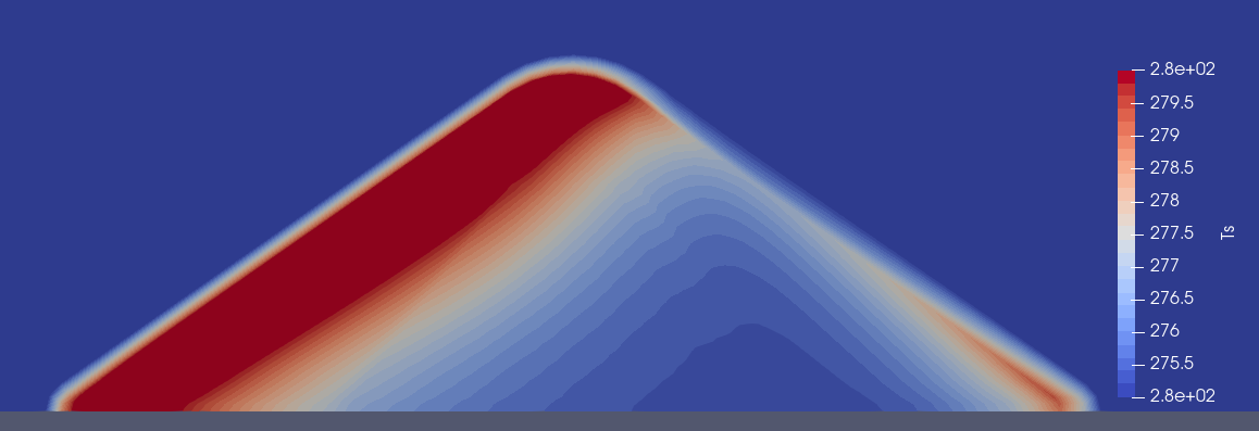
To see how this approach plays out, the solver is temporarily modified so that the PIMPLE loop is excluded (which throws a warning during compilation about an unused variable (cumulativeContErr), but which still seems to work). dt is set to 120. The initial conditions are then taken as a case that was previously solved with pimpleFoam and has a steady p and U field. The fields for the temperature equation are imported from an old CASE/0 folder. Here are three examples of the results, and they all look pretty OK:

U = 0.1 0 0, Laplacian included, Ks = 0.554, Asf = 0. 12 hours of simulation, with logs recorded at 15 minute intervals. Ts would previously have stopped climbing at around 1 second into this video.

U = 0.1 0 0, Laplacian included, Ks = 0.554, Asf = 30.04. 12 hours of simulation, with logs recorded at 15 minute intervals. I wouldn’t have previously bothered trying to run this model, knowing diffusion was so wrong. Scale of Ts as above.

U = 5 0 0, Laplacian included, Ks = 0.554, Asf = 30.04, Tf = 285. 12 hours of simulation, with logs recorded at 15 minute intervals. I wouldn’t have previously bothered trying to run this model, knowing diffusion was so wrong. NB: scale of Ts is very different in this animation compared to the two above.

Run times where also super quick – around 0.5 seconds for 12 hours, when p and U where already given.

A LIMITATION

Taking p and U as fixed means that dt was not restricted by the stability criteria defined by the Courant number (CFL criteria?).

SUGAR BEET CLAMP CFD MODELLING: A STRATEGY FOR DEALING WITH PRECISION ISSUES